Principles of Microeconomics
Beta
Start Recording
00:00:00
Tasks
Key points will be available post recording
Lecture Script

Transcripts will be available once the recording begins

Beta
Voice Notetaker

Voice Notetaker

Press to start
Microeconomic Principles
1. Introduction
Consumer Behavior Overview
2. Consumer Preferences
Rationality Properties
Utility Functions
Indifference Curves
Marginal Rate of Substitution
3. Budget Constraints
Budget Line and Equation
Impact of Income/Price Changes
4. Optimal Choice
Maximizing Utility
Marginal Utility & Principle
Corner Solutions
exam highlighterkey points
Full screen
  1. 1.
    Theory of Consumer Behavior
  2. 2.
    Basic Properties of Preferences
  3. 3.
    Utility and Preferences
  4. 4.
    Indifference Curves
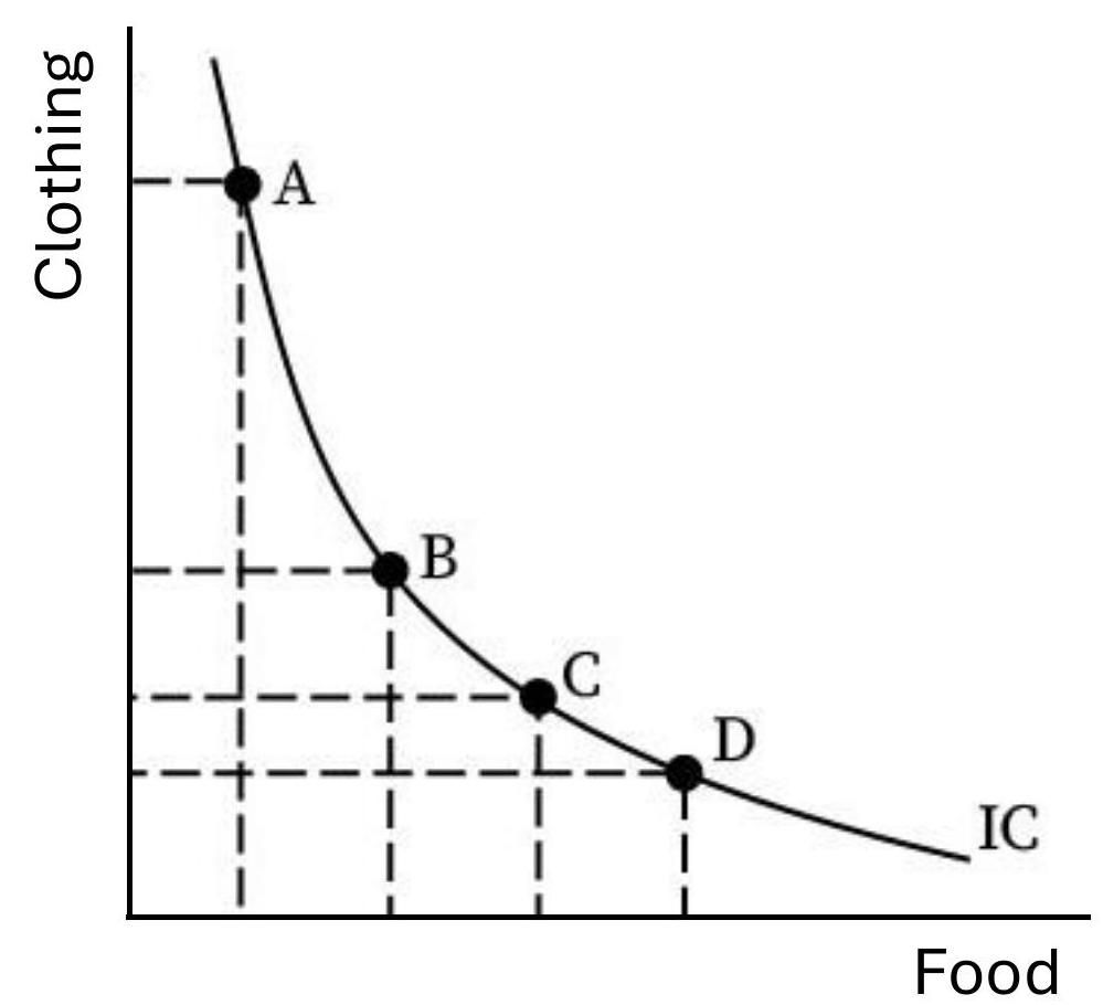
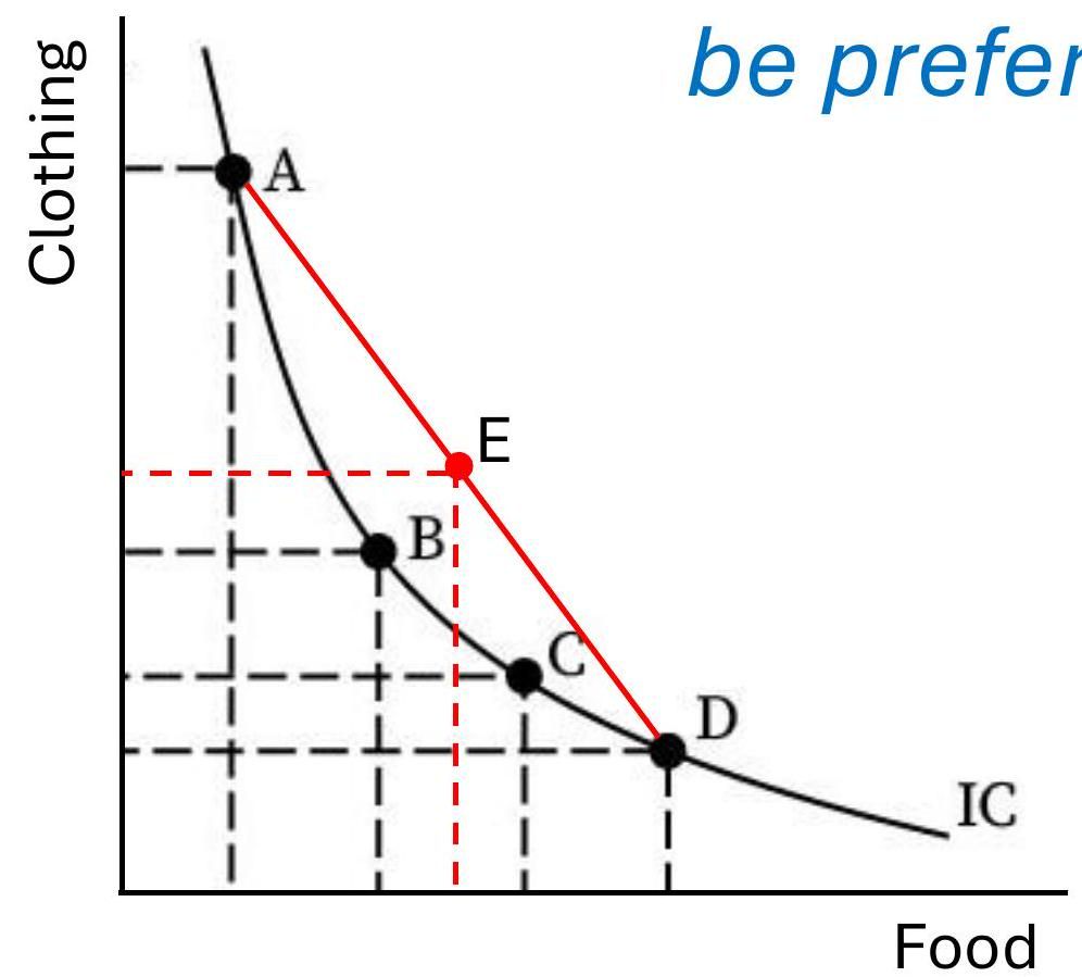
    • Indifference Curve; The graph shows an indifference curve (IC) representing different combinations of food and clothing that provide the same level of satisfaction to a consumer. Points A, B, C, and D represent different combinations of food and clothing on the indifference curve.
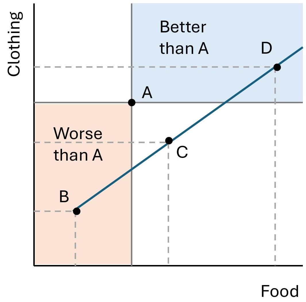
    • Production Possibilities Frontier; This figure shows a production possibilities frontier (PPF) for a hypothetical economy that produces only food and clothing. The PPF shows the maximum amount of one good that can be produced for every level of production of the other good. The slope of the PPF represents the opportunity cost of producing one good in terms of the other.
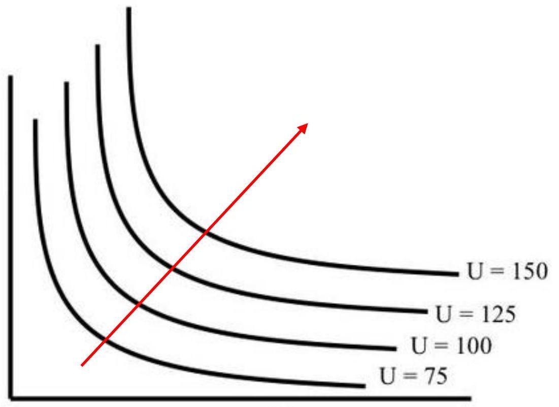
    • Potential Energy Contours; The graph shows potential energy contours for a system. The red arrow indicates the direction of decreasing potential energy, which is also the direction of the force acting on the system.
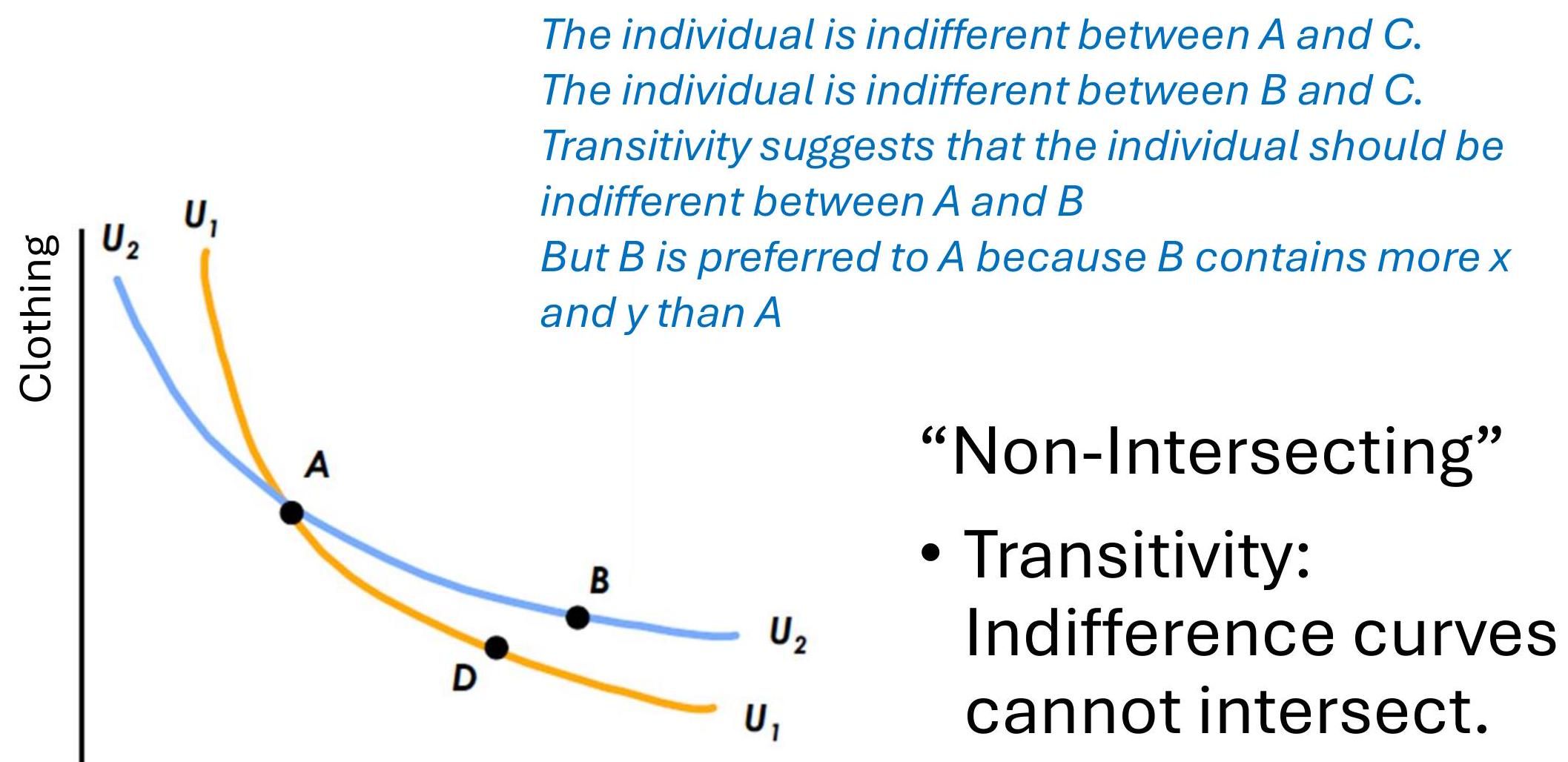
    • Indifference Curves; The figure shows two indifference curves, U1 and U2, which represent different levels of utility for an individual. The curves are labeled with points A, B, C, and D, which represent different combinations of goods. The curves are non-intersecting, which illustrates the concept of transitivity in consumer theory.
    • Indifference Curve; The indifference curve (IC) shows all the combinations of food and clothing that provide the same level of utility to the consumer. Point E represents the optimal consumption bundle, where the budget line is tangent to the indifference curve.
  5. 5.
    Marginal Rate of Substitution (MRS)
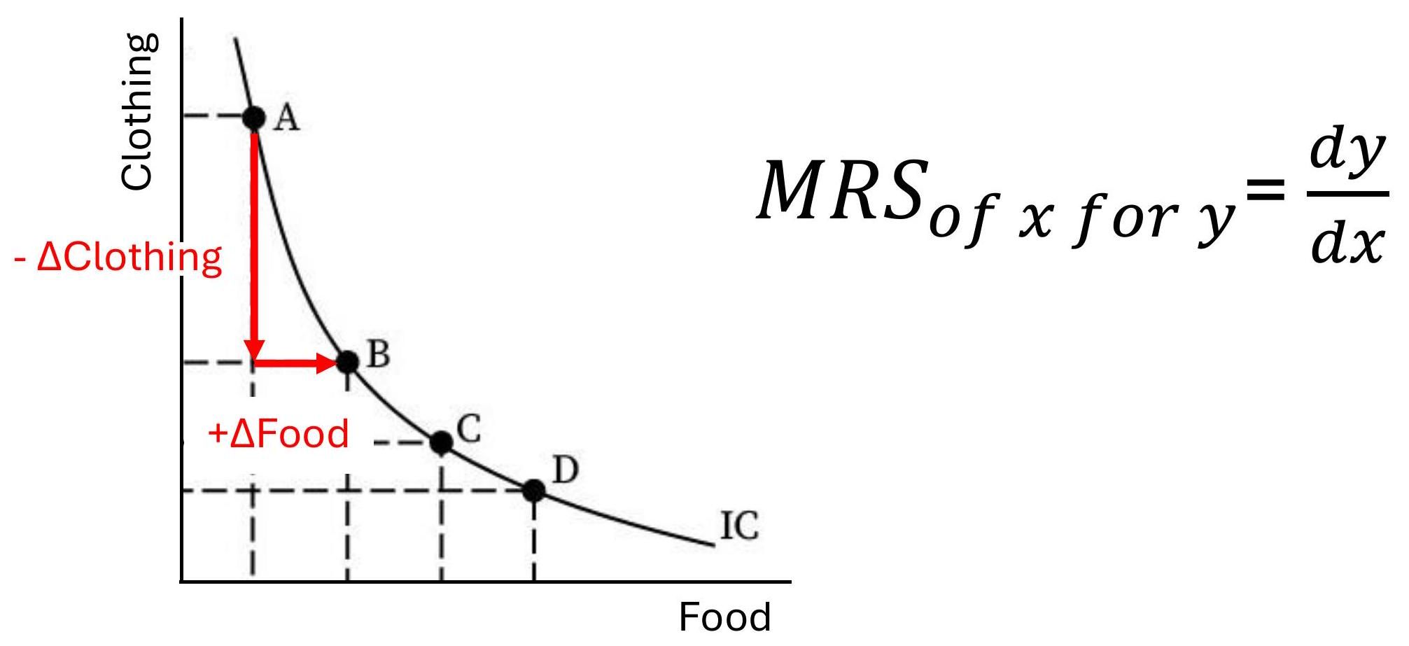
    • Indifference Curve; The figure shows an indifference curve (IC) with two goods, food and clothing. The slope of the indifference curve at any point represents the marginal rate of substitution (MRS) of food for clothing, which is the amount of clothing a consumer is willing to give up to get one more unit of food.
  6. 6.
    Budget Constraints
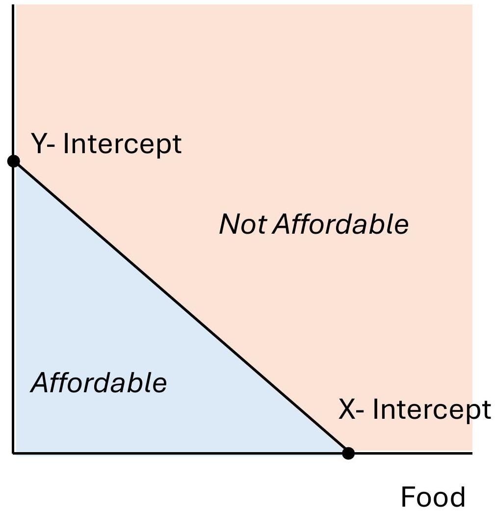
    • Budget Constraint; This figure shows a budget constraint, which represents all the combinations of two goods that a consumer can afford given their income and the prices of the goods. The area below the budget constraint line represents the affordable combinations, while the area above the line represents the combinations that are not affordable.
  7. 7.
    The Optimal Choice
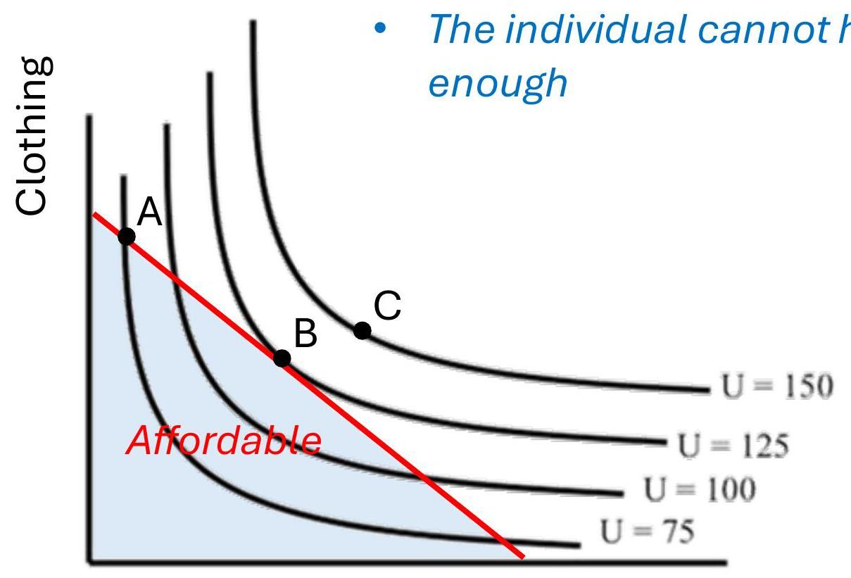
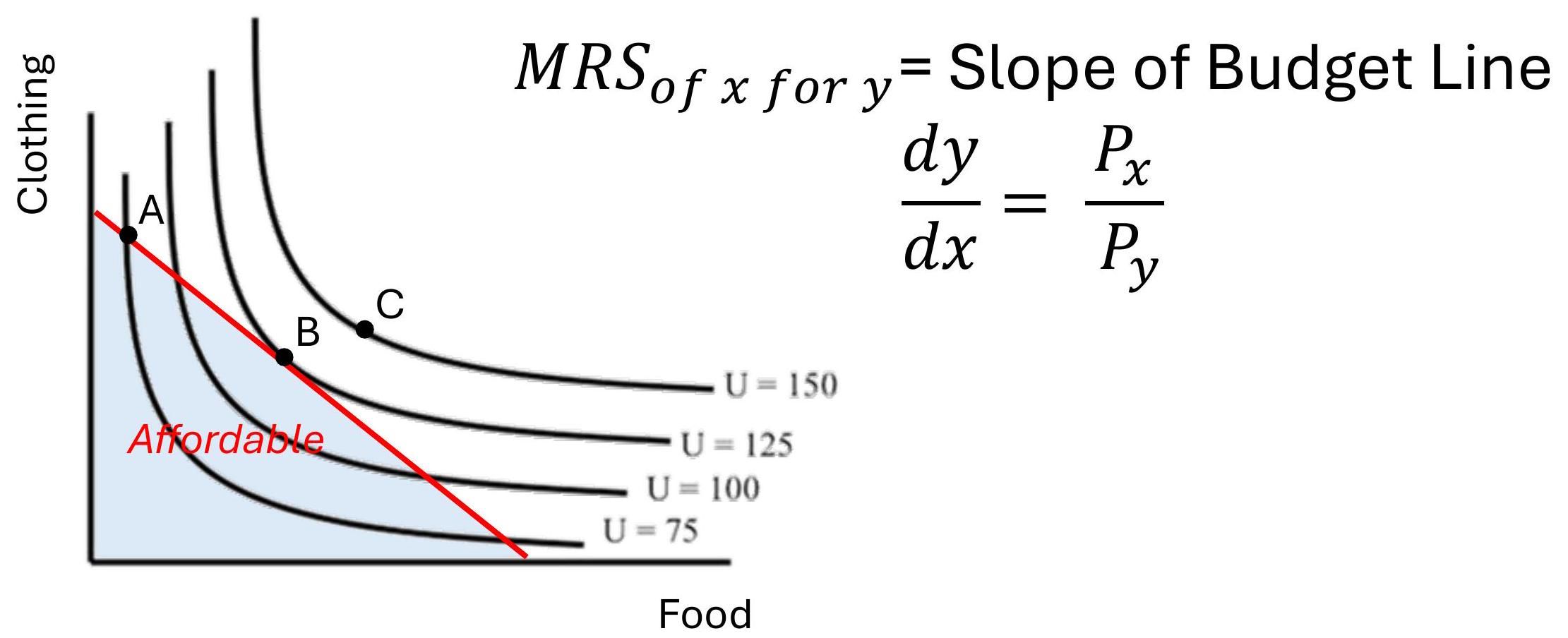
    • Indifference Curve and Budget Constraint; This figure shows indifference curves, which represent different levels of utility, and a budget constraint, which represents the combinations of goods that a consumer can afford. The point where the budget constraint intersects the highest indifference curve represents the optimal consumption bundle.
    • Indifference Curves and Budget Line; The figure shows indifference curves for different levels of utility (U) and a budget line. The slope of the budget line represents the price ratio of the two goods, while the slope of the indifference curve represents the marginal rate of substitution (MRS). The optimal consumption bundle is where the budget line is tangent to the highest attainable indifference curve.
  8. 8.
    Corner Solution
Ask to AI tutor
/
1